Handcrafted CNN from scratch - convolutional layer
This repo is inspired by my undergrad homework. The training speed was improved by 60x after refactoring the code. This article aims to illustrate how I used dot product instead of loops to perform forward/backward computations in convolutional layers.
Handling with batch data across multiple channels typically demands the extensive use of loops, and such loops significantly lead to slower training speed. With tensor dot products, these computations can be carried out all at once with parallel computation.
The full code is accessible here.
Features
- Fast tensor dot product operation provided by NumPy instead of for loops.
- Flexible, adaptive layer implementations allow customized network architectures.
Forward propagation
The shape of the features in the CNN is denoted as (batch size, channel size, height, width). The convolution operation in the convolution layer is carried out as follows.
The size of the output feature map after applying a convolutional layer to the input data can be determined using the following formula
output_size = (input_size - kernel_size + 2 * pad_size) / stride + 1
Since the value of stride is typically one, the formula can be simplified as follows.
output_size = input_size - kernel_size + 2 * pad_size + 1
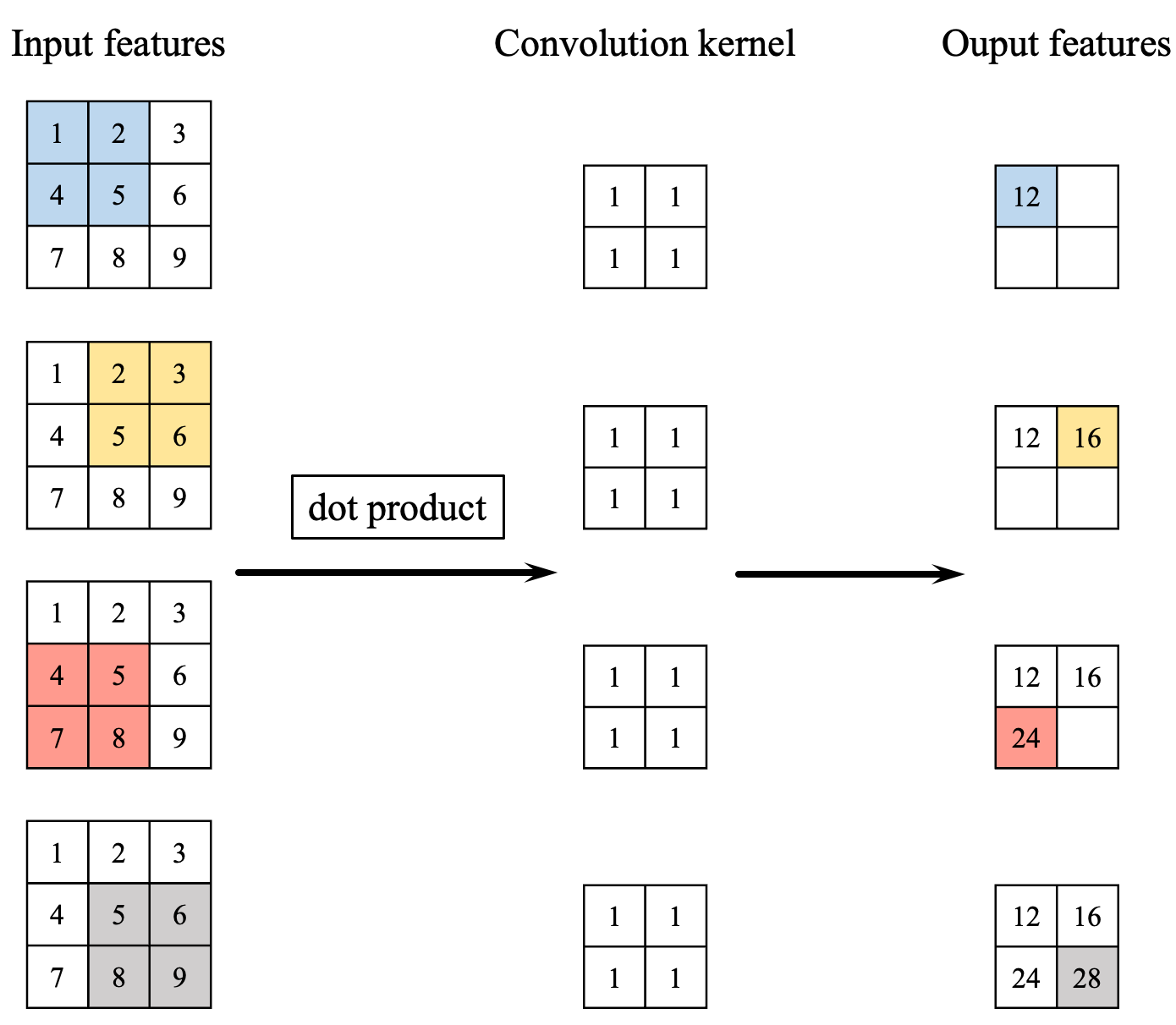
As illustrated in Figure 1, the forward propagation of a convolutional layer is essentially the dot product operation of the convolutional kernels on different windows in input features. Each of these dot products between the convolution kernel and input features can be accomplished using a loop. Furthermore, when we take into account different batches and channels of input data, we would need two more for loops. Hence, implementing forward propagation of the convolutional layer using loops can involve 3-6 nested loops. Fortunately, these loops can be avoided through the use of tensor dot products. Here's how I did it.
First, I use the function view_as_windows to make the windows that are to be used for dot product computations.
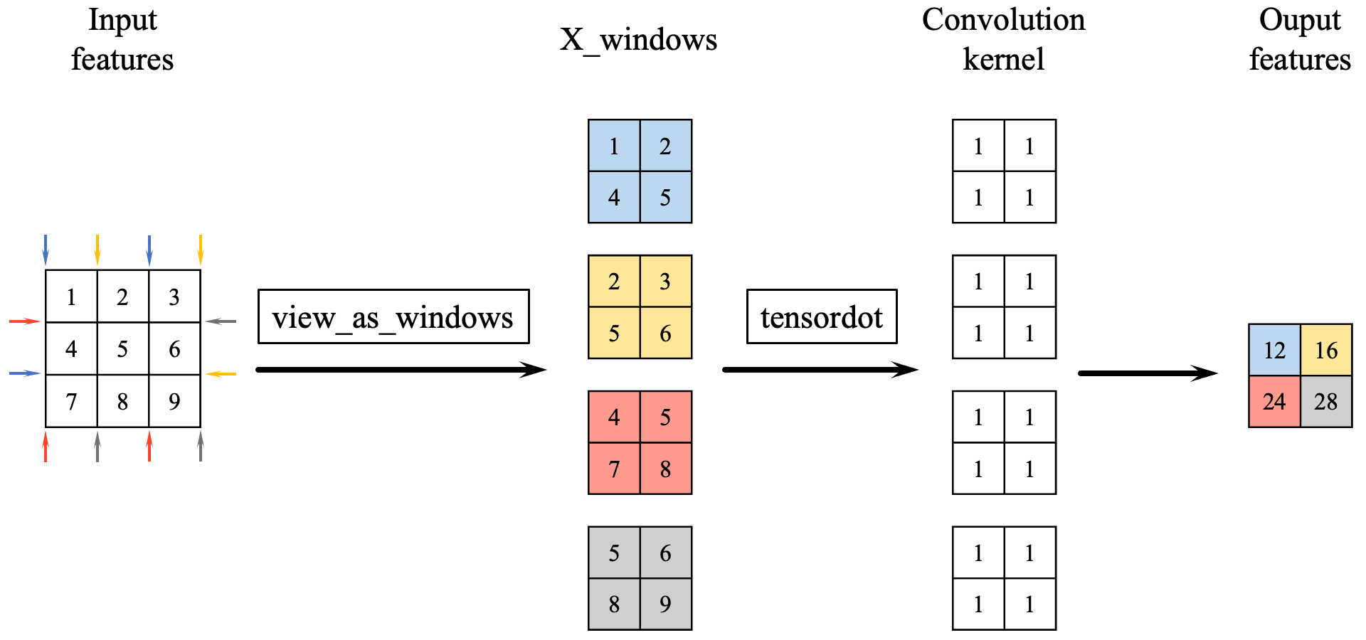
As demonstrated in the figure above, the role of view_as_windows function is to format data into a window structure for dot product operations, resulting in the tensor X_windows. Considering batch size and channel size, this function molds the features into a tensor with the shape (batch size, input channel size, output height, output width, kernel height, kernel width). The 4th and 5th dimensions (i.e., kernel height, kernel width) form the windows that will undergo dot product with the convolutional kernels, while the 1st dimension represents the number of channels in the input features.
The next step is to perform a tensor dot product with convolutional kernel W, which has a shape of (output channel size, input channel size, kernel height, kernel width). The 1st, 2nd, and 3rd dimensions of W (i.e., input channel size, kernel height, kernel width) should match with the corresponding axes of the input features, ensuring that the dot product is carried out along the correct axes of the kernel and the features. After the tensor dot product, bias b is added to this tensor, yielding the output features with a shape of (batch size, output channel size, height, width).
The code for the forward propagation computation is as follows, which matches exactly with the description above. In addition, the following code also includes the padding.
def forward(self, X):
    # input shape
    batch_size, in_ch_size, in_H_size, in_W_size = X.shape
    # weight shape
    _, _, Wx_size, Wy_size = self.W.shape

    # determine the output dimensions
    out_H_size = in_H_size - Wx_size + 1 + 2 * self.pad_size
    out_W_size = in_W_size - Wy_size + 1 + 2 * self.pad_size

    # pad the input
    padding = [(0, 0), (0, 0), (self.pad_size, self.pad_size), (self.pad_size, self.pad_size)]
    X_padded = np.pad(X, padding, mode='constant')

    # create X_windows for conv operation
    window_shape = (1, 1, Wx_size, Wy_size)
    view_window_stride = 1
    X_windows = view_as_windows(X_padded, window_shape, view_window_stride)
    X_windows = X_windows.reshape(batch_size, in_ch_size, out_H_size, out_W_size, Wx_size, Wy_size)

    # perform convolution operation
    out = np.tensordot(X_windows, self.W, axes=([1,4,5], [1,2,3]))
    # (batch_size, out_H_size, out_W_size, out_ch_size) -> (batch_size, out_ch_size, out_H_size, out_W_size)
    out = np.transpose(out, (0, 3, 1, 2))
    out += self.b

    return out
Backward propagation
There are three gradients that need to be calculated in backpropagation phase: the gradient w.r.t convolution kernel dL/dW, the gradient w.r.t bias dL/db, and the gradient w.r.t input feature dL/dX. The gradient of the convolution kernel is the convolution of the upstream gradient (i.e., the gradient of the loss function w.r.t the output of this layer) and input features, while the gradient of the bias is the sum of the upstream gradient. These two gradients are used to update the kernel and bias respectively.
The following figure demonstrates the calculation of backpropagation for the input feature.
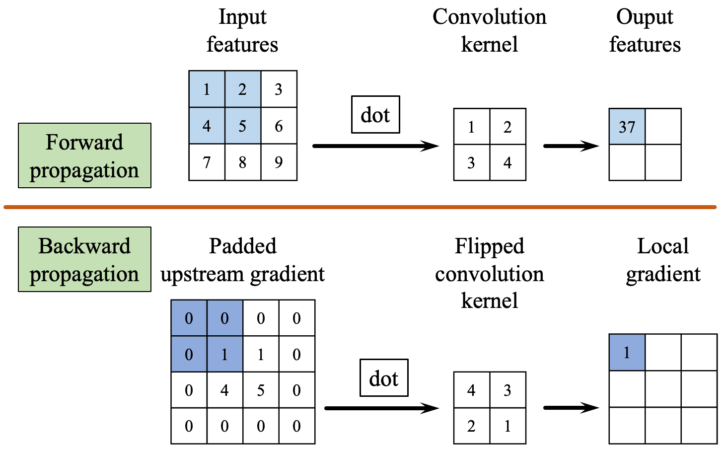
Before computing the gradient w.r.t the input, padding needs to be applied to the upstream gradient to ensure that the shape of the result from the convolution operation during backpropagation aligns with the shape of the input. The amount size of padding (or unpadding) can be obtained as follows:
unpad_size = kernel_size - pad_size - 1
After applying padding to the upstream gradient, it undergoes convolution with the flipped weight tensor W_flipped to yield the gradient w.r.t the inputs of this layer. Therefore, the implementation for the backward propagation is as follows.
def backprop(self, dLdy):

    # reshape dLdy to (batch_size, ch_size, out_H_size, out_W_size)
    # since the shape of dLdy may be (batch_size, ch_size * out_H_size * out_W_size)
    dLdy = dLdy.reshape(self.fwd_cache["out_shape"])

    # load the cache data
    X = self.fwd_cache["X"]
    X_padded = self.fwd_cache["X_padded"]
    pad_size = self.pad_size

    # input shape
    batch_size, in_ch_size, in_H_size, in_W_size = X.shape
    # weight shape
    out_ch_size, _, Wx_size, Wy_size = self.W.shape

    # determine the output dimensions
    out_H_size = in_H_size - Wx_size + 1 + 2 * pad_size
    out_W_size = in_W_size - Wy_size + 1 + 2 * pad_size

    # create X_windows for conv operation
    window_shape = (1, 1, Wx_size, Wy_size)
    view_window_stride = 1
    X_windows = view_as_windows(X_padded, window_shape, view_window_stride)
    X_windows = X_windows.reshape(batch_size, in_ch_size, out_H_size, out_W_size, Wx_size, Wy_size)

    # gradient w.r.t. weights
    dLdW = np.tensordot(dLdy, X_windows, axes=([0,2,3], [0,2,3]))

    # gradient w.r.t. bias
    dLdb = np.sum(dLdy, axis=(0,2,3)).reshape(1, out_ch_size, 1, 1)

    # gradient w.r.t. inputs
    # create dLdy_windows for conv operation
    # calculate unpad_size used in backprop
    unpad_size_H = Wx_size - pad_size - 1
    unpad_size_W = Wy_size - pad_size - 1
    dLdy_padded = np.pad(dLdy, ((0, 0), (0, 0), (unpad_size_H, unpad_size_H), (unpad_size_W, unpad_size_W)), mode="constant", constant_values=0)
    dLdy_windows = view_as_windows(dLdy_padded, window_shape, view_window_stride)
    dLdy_windows = dLdy_windows.reshape(batch_size, out_ch_size, in_H_size, in_W_size, Wx_size, Wy_size)
    # create flipped W, i.e., rotate self.W 180 degrees
    W_flipped = self.W[..., ::-1, ::-1]

    # perform convolution operation, same as forward propagation
    dLdx = np.tensordot(dLdy_windows, W_flipped, axes=([1,4,5], [0,2,3]))
    dLdx = np.transpose(dLdx, (0, 3, 1, 2))

    return dLdx, dLdW, dLdb